Metrology: III - Navigating the Uncertainty: Understanding the Significance of Measurement Uncertainty in Scientific Analysis

In our previous post we defined uncertainty as a ‘non-negative parameter characterizing the dispersion of the quantity values being attributed to a measurand, based on the information used.’ (source: VIM). Quite a bland statement, even though perfectly correct. So what exactly is uncertainty?

Let’s take a look.

Measurement uncertainty

In the broadest metrological terms, uncertainty is the doubt that exists about the result of any measurement.

It is important to distinguish between uncertainty and error. While an error is the difference between the measured value and the ‘true’ value, uncertainty is a quantifiable doubt (expressed in statistical terms) about the measurement.

To enhance the amount of information gleaned from your measurements, the wisest approach is taking multiple readings and employing fundamental statistical computations. The primary calculations to focus on are determining the average or arithmetic mean and calculating the standard deviation for a given set of numbers.

An average or arithmetic mean is usually shown by a symbol with a bar above it, e.g. x̄ (‘x-bar’) is the mean value of x. In general, it is advisable to perform as many readings as possible for a given measurement, however, adding readings has (thankfully) diminished results. For accurate measurements, at least 10 readings are advised but, depending on the length and complexity of the measurement, this is not always possible. An absolute minimum of at least three readings should, however, be employed in all cases.

Standard deviation is the most general way of defining the “spread” of the measurement across the range of measurement readings. The standard deviation of a group of numbers provides insight into the typical variation of individual readings from the set's average. The true standard deviation value can only be derived from an extensive (infinite) collection of readings. When dealing with a moderate number of values, only the estimated the standard deviation is attainable, typically denoted by the symbol "s."

Sources of uncertainties and errors

• Measuring instruments, which can be affected by errors including bias, changes due to aging, wear, drift, poor readability, and noise.
• The item being measured, which might not be stable, as seen when measuring the size of an ice cube in a warm room.
• The measurement process itself can be challenging, especially when dealing with small but lively animals or difficult-to-measure objects.
• 'Imported' uncertainties can also play a significant role in certain measurements, affecting setup, fine detail reading, and reaction times.
• Operator skill and judgment can arise if the measurements are not representative of the process being assessed.
• Sampling issues
• The environment's conditions, such as temperature, air pressure, and humidity, can impact both the measuring instrument and the item being measured.

Types of uncertainties

Like measurement errors, uncertainties can also be categorized as random and systematic. The definition of each type is as follows:

• Random uncertainty yields randomly different results upon repeating measurements, and averaging multiple measurements generally leads to a better estimate.
• Systematic uncertainty is characterized by a consistent influence affecting each repeated measurement and is often undetectable without additional methods for estimation.

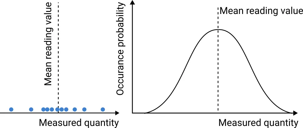
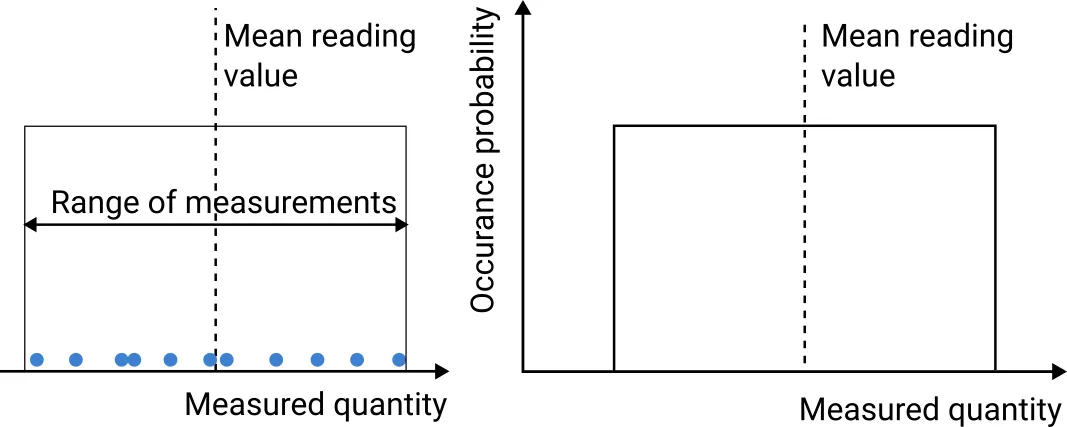
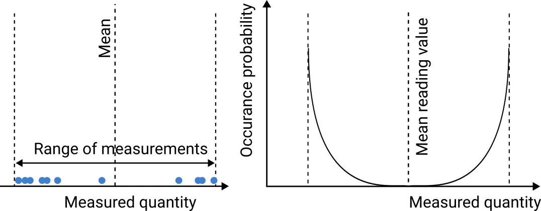
In terms of probability distribution, measurement uncertainty can take many different shapes. These fall somewhere between the following three theoretical distributions:

1. Gaussian or normal distribution
2. Rectangular distribution
3. U-shaped distribution




Fig. 1. Gaussian normal distribution



Fig. 2. Rectangular distribution



Fig. 3. U-shape distribution

Propagation of uncertainty

An additional concept we need to consider in uncertainty analysis is the so-called propagation of uncertainty (or propagation of error). Put simply, propagation of uncertainty defines how uncertainties in the input quantities of a mathematically calculated resultant quantity influence the uncertainty in the final output. It helps us grasp how small errors in the initial data can impact the accuracy of our end result, commonly applied in scientific and engineering disciplines to ensure precise calculations and predictions.

How to evaluate uncertainty?

The Guide to the Expression of Uncertainty in Measurement (or GUM) defines two methods of uncertainty evaluation:

• Type A evaluation - uncertainty estimates based on repeated measurements and suitable statistical probability distribution as just described
• Type B evaluation - uncertainty assessed based on other available information which encompass past experience, validated models, calibration certificates and other relevant knowledge about the measured quantity. This information can help us define boundaries or specific ranges inside which a specific parameter of the measurement can influence the overall result. (Inside these ranges, various distributions functions can again be assumed to ‘model’ the influence of the parameter in question.)

While Type A can be thought of as the general by-the-book method of assessing uncertainty, the Type B method can often help improve the measurement quality rather substantially.

To evaluate uncertainty, there are several key steps we need to follow:

1. Define a test protocol with information you want to obtain from the measurements, the range of measurements required, and calculations needed for the final results
2. Execute the measurements
3. Estimate individual uncertainties
4. Decide if the uncertainties are independent of one another
5. Calculate the final result
6. Evaluate the combined uncertainty based on the input quantity uncertainties
7. Define the combined uncertainty using coverage factor, size of the uncertainty interval and a level of confidence
8. Report the measurement result with the evaluated uncertainty along with the used measurement and evaluation methodology

These steps will be discussed more in detail in the example presented below.

Main terms and parameters to consider when calculating uncertainty

Standard uncertainty

Each individual uncertainty contributing to the combined uncertainty of the measurement has to be expressed at the same level of confidence as standard uncertainties.

To this end, the standard uncertainty is typically used, which is expressed as a ± margin value that is the size of one standard deviation

The symbol u is generally used for expressing standard uncertainty.

Type A standard uncertainty

The Type A standard uncertainty can be expressed as:

\begin{multline} \shoveleft u = {s \over \sqrt{N}}, \end{multline}

where \(s\) is the standard deviation and \(N\) is the number of recordings per measurement.

Type B standard uncertainty

In instances of limited information, particularly in Type B estimates, one may need to estimate both upper and lower uncertainty bounds, assuming an equal likelihood of the value falling anywhere in between, resulting in a rectangular or uniform distribution. In this case:

\begin{multline} \shoveleft u = {a \over \sqrt{3}}, \end{multline}

where \(a\) is the half width of the (expected) measurement deviation limits.The selection of the type of distribution is down to the specifics of the test setup and the available knowledge about the specific type of uncertainty being analysed. One can, e.g., generally presume that uncertainties derived from the calibration certificate of a measuring instrument follow a normal distribution.

Combined standard uncertainty

In the simplest case, a measured quantity hold several independent measurement uncertainties (e.g. Type A uncertainty and several Type B uncertainties deriving from the used measurement setup). In this case, the combined uncertainty is:

\begin{multline} \shoveleft u_c = \sqrt{u_a^2+u_b^2+...+u_X^2} \end{multline}

For more complex cases with quantities derived from equations with multiple different units, refer e.g. to UKAS, The Expression of Uncertainty and Confidence in Measurement M 3003.

Individual uncertainties correlation

Often, uncertainties are independent of one another. If, however, this is not the case, then the uncertainty analysis becomes somewhat more involved. Refer again to the UKAS handbook or to the sources at the end of this article to find out more

Coverage factor \(k\)

If one wishes to express the combined standard uncertainty at a different confidence level, such as, e.g., 95 %, re-scaling is achieved by multiplying the combined standard uncertainty (\(u_c\)) by a coverage factor (\(k\)). The result is known as the expanded uncertainty (\(U\)), and a specific coverage factor corresponds to a particular confidence level. The most commonly used coverage factor is \(k = 2\), providing an approximate 95-% confidence level, assuming the combined standard uncertainty is normally distributed. Different coverage factors, such as \(k = 1\), \(k = 2.58\), and \(k = 3\), correspond to confidence levels of approximately 68 %, 99 %, and 99.7 %, respectively, in a normal distribution, while other distributions have unique coverage factors.

Example: CMM measurement of an aluminum block’s length

Suppose we want to measure the length of an aluminum block using a coordinate measuring machine (CMM). To measure the length of the aluminum block, we would first place it on the CMM's table and align it using the CMM's software. Then, we would use the CMM's touch probe to measure the distance between two points on the aluminum block.



Fig. 4. CMM measurement probe (symbolic image)

During the procedure, various possible errors can occur:

• CMM errors:
• Probe tip error
• Linear axis error
• Volumetric error
• Thermal error
• Aluminum block errors:
• Thermal expansion
• Surface finish
• Alignment errors
• Measurement process errors:
• Operator error
• Environmental conditions (temperature, humidity, vibration, etc.)
• Other possible errors:
• CMM software errors
• Aluminum block material properties (e.g., hardness, elasticity)
• CMM calibration status

First, let's look at some possible actions to mitigate measurement errors:

1. Use a calibrated CMM with a known error budget.
2. Use a touch probe with a sharp tip and a small diameter
3. Measure the aluminum block at a constant temperature
4. Place the aluminum block on the CMM's table in a stable and aligned position
5. Use the CMM's software to compensate for thermal expansion and other errors
6. Have the measurement performed by a trained operator.

Typically, the CMM's software would automatically calculate the length and the uncertainty of the measurement. To mitigate errors, we would make sure that the CMM is calibrated and that the temperature in the CMM lab is constant. We would also use a trained operator to perform the measurement. Even after mitigation of most possible sources of error, the measurement will still no doubt exhibit a degree of uncertainty. Let's analyze and report it following the steps noted above.

Step 1. Define test protocol, i.e., decide what you need to find out from your measurements and what are the possible sources of the measurement errors.

• Measured quantity: length of an aluminum block
• Possible errors
• CMM device:
• Stated calibration accuracy
• Resolution of the A/D conversion
• Measured item:
• Damage on the sample
• Ductility of the material influences the measurement
• Thermal expansion
• Operator:
• Incorrect positioning of the measured sample
• Other

Step 2. Measurement execution

The measurement of the block is repeated N times (N=3 being the absolute minimum). After the measurement, the mean value and the standard deviation are evaluated. The measurement should include the following info:

• Date/Time of measurement
• Exact measurement method (sample position, type of tip, etc.)
• Environmental conditions
• Anything else relevant to the measurement

In our example we obtained the following data:

• Average measurement 10.521 mm (N=3)
• Standard deviation: 2.2 µm

Step 3. Estimate the individual uncertainties

Type A uncertainty

The Type A uncertainty is calculated based on the evaluated standard deviation as:

\begin{multline} \shoveleft u = {s \over \sqrt{N}} =1.27\ \mathrm{µm} \end{multline}

Type B uncertainty

Let’s suppose the calibrated CMM has a 0.05% uncertainty, which, for an average measurement of 10.521 mm, results in 5.261 µm. At a coverage factor k = 1, this results in a standard uncertainty of:

\begin{multline} \shoveleft u = 2.63\ \mathrm{µm}, \end{multline}

which is the half width of the stated uncertainty range.

The resolution of the device is ±0.3 µm, which can be considered a linearly distributed uncertainty. The standard uncertainty in this case is

\begin{multline} \shoveleft u = {0.3 \over \sqrt{3}} = 0.173\ \mathrm{µm} \end{multline}

The sample mounting system can additionally yield excessive clearance of up to 0.01 mm. Assuming a uniform distribution of the clearances on the samples measured, the standard uncertainty is:

\begin{multline} \shoveleft u = {0.01 \over 2}\cdot{1 \over \sqrt{3}} = 2.9 \ \mathrm{µm} \end{multline}

Step 4. Decide if the uncertainties are independent of one another

For the described case we assume the quantities are independent.

Step 5. Calculate the final result

The average measurement was 10.521 mm. Just for example purpose, let’s assume that the measurement included an additional gauge block of 0.5 mm (with negligible uncertainty below 0.1 µm) that had to be added for mounting purposes. The gauge length has to be excluded from the result, so the average measurement is 10.021 mm.

Step 6. Evaluate the combined uncertainty based on the input quantity uncertainties

The combined uncertainty can be evaluated by using the equation described in the previous section as:

\begin{multline} \shoveleft u_c = \sqrt{1.27^2+2.63^2+0.173^2+2.9^2} = 4.1\ \mathrm{µm} \end{multline}

Step 7. Define the combined uncertainty using coverage factor, size of the uncertainty interval and a level of confidence

Considering a coverage factor k = 2, which translates to a confidence level of 95%, the expanded uncertainty is 8.1 µm.

Step 8. Report the measurement result with the evaluated uncertainty along with the used measurement and evaluation methodology

Write the result in a similar form to the following.

Gauge block length: 10.021 ± 0.0081 mm (expanded uncertainty evaluated as standard uncertainty times the coverage factor k = 2)

Block length is the average of 3 measurements corrected to exclude added gauge block length. Uncertainty measured according to the method defined in [source].

Conclusion

Measurement uncertainty is an integral component of scientific research, influencing the reliability, reproducibility, and credibility of empirical findings. Embracing robust mathematical frameworks and implementing advanced calibration and validation protocols are crucial for mitigating the adverse effects of uncertainty on experimental outcomes. By fostering a culture of transparent communication and continually refining uncertainty assessment methodologies, the scientific community can bolster the trustworthiness and applicability of research findings, thereby paving the way for more accurate and dependable scientific discoveries and applications.




References

[1] S. Bell, A Beginner's Guide to Uncertainty of Measurement, Issue 2

[2] 2006 IPCC Guidelines for National Greenhouse Gas Inventories, Volume 1 General Guidance and Reporting, Ch. 3, Uncertainties

[3] United Kingdom Accreditation Service, M3003, The Expression of Uncertainty and Confidence in Measurement

Back to blog Go to next post